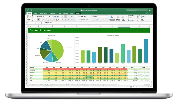
Excel is quite possibly the most useful application that is sitting on your computer not doing much at all. While it can be used for things like holiday packing check lists, where it really flexes its muscles is in transforming numbers, for instance doing your Christmas budget, calculating how much you can put towards your mortgage, or keeping track of fundraising for your local school.
Excel sheets are in the form of a table. Each small rectangle in Excel is known as a cell. Each cell is identified by a unique letter and number you can find at the top and left of your table. Today we run through some very handy formulas you can put in a cell that will transform the data of other numeric cells.
In these formula examples, we use the form (LETTERNUMBER, LETTERNUMBER) which means you are using all the cells –- separated by commas figure out the formula. This list can have one item or many items. You can also have it in the form of (ANUMBER:ANUMBER) for continuous row selection – row A in this case, or (LETTER4:LETTER4) for continuous column selection – column 4 here.

Add all numbers together
=SUM(A2,A15)
For example, if the number 32 is in cell A2, and the number 48 is in A15, if you type =SUM(A2,A15) in another cell and press enter, it will then display as 80.
Average of all numbers
=AVERAGE(B4,B9,B12)
Let’s say that the number 11 is in cell B4, the number 15 is in B9, and the number 4 is in B12. When you type =AVERAGE(B4,B9,B12) in another cell then press enter, the cell will then display as 10.
Maximum from list of numbers, minimum from list of numbers
=MAX(B4,B9,B12) & =MAX(B4,B9,B12)
Let’s work with the same cells and values as the above example, (11 is in cell B4, 15 is in B9, and 4 is in B12). Typing =MAX(B4,B9,B12) in another cell and pressing enter will then show the result: 15. If you type =MIN(B4,B9,B12) it will display 4 as the result instead.
Count of numbers entered
=COUNT(C2,C7,C17)
This example just counts the number of cells with numbers in them. If C2 has 34 in it, C7 has the word “tomorrow” in it, and C17 has 9 in it, then typing =COUNT(C2,C7,C17) in another cell and pressing enter will give you 2 as the result.
Round up number, round down number
=CEILING(C3,significance) & =FLOOR(C3, significance)
Need to round things to the nearest whole number, nearest 0.01? This will do it for you – rounding up or down. If we have 11.009 in C3, and then enter =CEILING(C3,0.01) in another cell, we will get 11.01 as the result. If we enter =FLOOR(C3,0.01) instead, then we will get 11 as the result.
Have some other Excel magic you’d like to share? Put it in the comments section to help others out!


Join the Discussion
Type out your comment here:
You must be logged in to post a comment.